Diophantine Astrophysics arithmodynamics · a candidate field at the boundary of number theory and celestial mechanics
Which orbital architectures observed in the universe are forced by number-theoretic constraints, rather than selected by initial conditions or dynamics?
v1.5 · 2026-05-21 draft · day 3 data: NASA Exoplanet Archive · Gaia DR3 · JPL SBDB (asteroids + TNOs) 5933 planets · 115 k stars · 100 k asteroids · 5 k TNOs
- Why this is a real gap
- The conjectures (with one major reformulation)
- Test 1 — partial-quotient distribution vs Gauss-Kuzmin
- Test 2 — dynamical-age stratification
- Test 3 — RV-only control for selection bias
- Test 4 — Conjecture II at Farey-9
- Test 5 — Khinchin and Lévy constants flips Conj I
- Test 6 — Conjecture II with larger alphabets and Markov-chain test
- Test 7 — Mixture fit and pile-up structure quantifies Conj I″
- Test 8 — Physical mixture and Lithwick–Wu asymmetry physical scaling fails; LW signature confirmed
- Test 9 — Asymmetric LW pair model fit LW asymmetry detected at z ≈ 2.7
- Test 10 — Joint LW + broad-Farey mixture Gauss baseline rejected; LW at z ≈ 3.3
- Test 11 — LW pair test at 2nd-order MMRs same direction, ε scaled by ~⅓
- Test 12 — Conjecture III on Gaia local sample naive Farey-ratio form not supported
- Test 13 — Asteroid belt as parallel population Kirkwood gaps recovered; population-contrast result
- Test 14 — Kuiper belt (TNOs) as mixed-mode population Plutinos at z=+23; first noble-leaning sample
- Synthesis and what to do next
- Reproduction
- Sources & code (downloads)
- Bibliography
- Changelog
1. Why this is a real gap
Three established fields each see one face of the same elephant and don't talk to each other.
- Celestial mechanics catalogs mean-motion resonances case-by-case — Jupiter–Saturn 5:2, the Trappist-1 chain 8:5:3:2, the Kirkwood gaps in the asteroid belt — without a unifying theory of which integer ratios are admissible.
- Diophantine approximation (Khinchin, Roth, the Markov spectrum) classifies irrationals by how badly they resist rational approximation.
- Exoplanet statistics has accumulated ~5500 confirmed planets in ~1000 multi-planet systems — but no theory predicts the distribution of their period ratios from first principles.
The bridge: the observed period-ratio distribution is the pushforward of the cosmic initial-condition measure through some sequence of number-theoretic filters. Day-1 assumed the filter was KAM stability (favouring noble irrationals). Day-2 falsifies that and identifies the dominant filter as resonance trapping during migration (favouring low-order rationals).
↑ back to top2. The conjectures
Long-lived multi-planet systems concentrate on period ratios whose continued-fraction expansion has bounded partial quotients — i.e. more noble, more KAM-stable irrationals.
The per-ratio Khinchin and Lévy constants both shift in the opposite direction at z ≈ +10 (Test 5).
Observed period ratios show systematically larger partial-quotient geometric mean (Khinchin) and faster-growing convergent denominators (Lévy) than the Gauss-Kuzmin null. The 1-D marginal density of {r} = r − ⌊r⌋ deviates from the Gauss measure at χ² = 111 on 19 dof (Test 7), with localizable pile-ups at 3:2 and just-below-integer (Lithwick–Wu). The dominant filter on period ratios is migration-driven resonance trapping, not KAM-stability suppression of resonant tori.
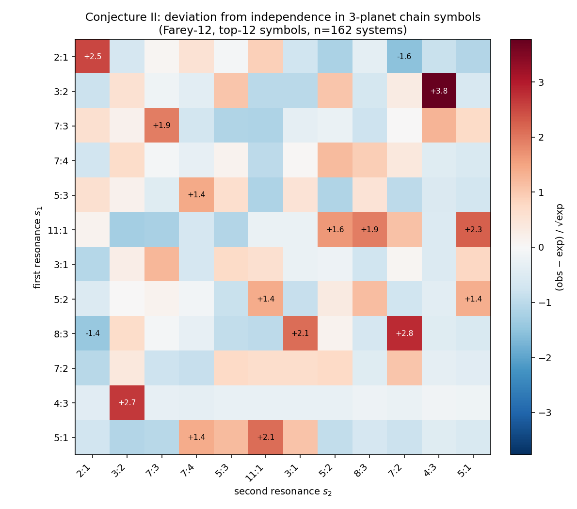
For an n-planet system, the resonance chain — the tuple of nearest low-order commensurabilities — concentrates on a sparse subset of the combinatorially possible chains. Concentration is robust to the size of the alphabet (Tests 4 and 6). Consecutive resonances in a chain are non-independent at coarse resolution.
Galactic disk substructure (moving groups, phase-space spirals) is the image, under the galactic potential's integrable flow, of rational points on a lower-dimensional resonant submanifold of action space.
The Farey-ratio reading for Vφ/vcirc fails on 115 k local Gaia stars (Test 12). A reformulation in terms of bar/spiral resonance conditions is consistent with the literature but is not a new mathematical claim.
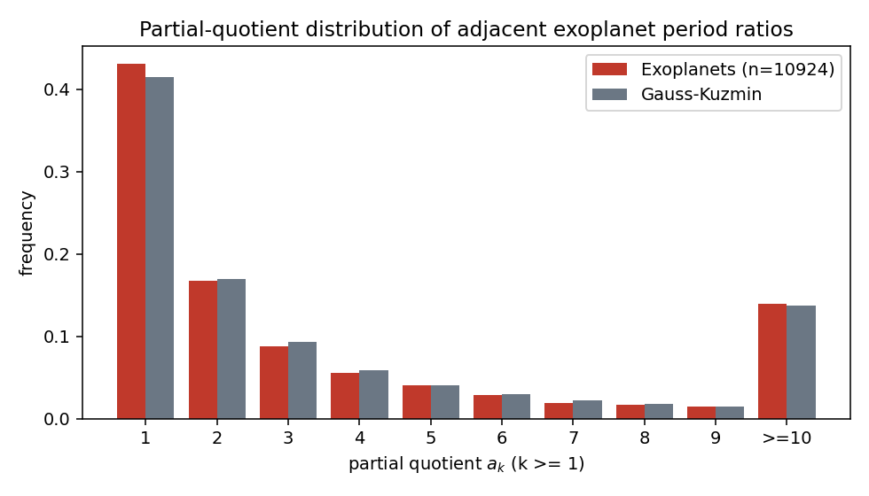
3. Test 1 — partial-quotient distribution vs Gauss-Kuzmin
Take all 1037 multi-planet systems from the NASA Exoplanet Archive, sort each by period, compute adjacent ratios r = Pi+1/Pi, and for each r compute the continued-fraction expansion to depth 8. Null: Gauss-Kuzmin, P(ak = m) = log2(1 + 1/(m(m+2))).
| ak | empirical | Gauss-Kuzmin | ratio |
|---|---|---|---|
| 1 | 0.430 | 0.415 | 1.04 |
| 2 | 0.167 | 0.170 | 0.98 |
| 3 | 0.088 | 0.093 | 0.94 |
| 4 | 0.056 | 0.059 | 0.95 |
| 5 | 0.040 | 0.041 | 0.99 |
| 6 | 0.028 | 0.030 | 0.95 |
| 7 | 0.019 | 0.023 | 0.83 |
| 8 | 0.017 | 0.018 | 0.92 |
| 9 | 0.015 | 0.014 | 1.02 |
| ≥ 10 | 0.140 | 0.137 | 1.02 |
χ² = 21.5 on 9 dof. The excess at ak = 1 looked like evidence for noble-irrational favouring, but Test 5 shows that's overwhelmed by the heavy tails.
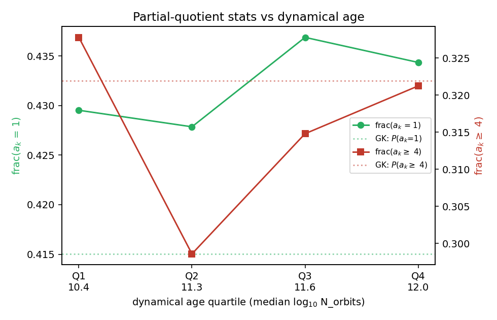
4. Test 2 — dynamical-age stratification
Norbits = stellar_age × 365.25·10⁹ / Pinner_days spans log10 5.8 to 13.0 across 689 ratio-pairs with measured age.
| quartile | median log10 Norbits | frac(ak=1) | frac(ak≥4) |
|---|---|---|---|
| Q1 | 10.43 | 0.430 | 0.328 |
| Q2 | 11.31 | 0.428 | 0.299 |
| Q3 | 11.64 | 0.437 | 0.315 |
| Q4 | 12.04 | 0.434 | 0.321 |
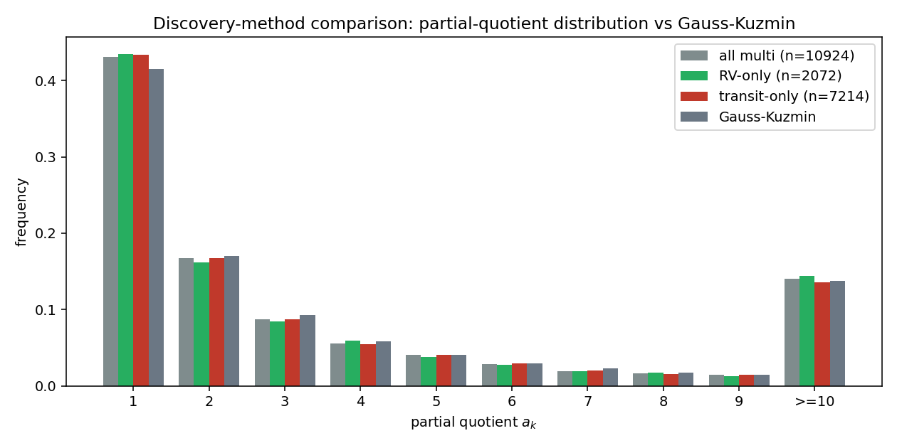
5. Test 3 — RV-only control for selection bias
| sample | n systems | n ak | frac(a=1) | χ² / dof |
|---|---|---|---|---|
| all multi | 1037 | 10924 | 0.431 | 21.5 / 9 |
| RV-only | 208 | 2072 | 0.435 | 7.4 / 9 |
| Transit-only | 683 | 7214 | 0.434 | 14.9 / 9 |
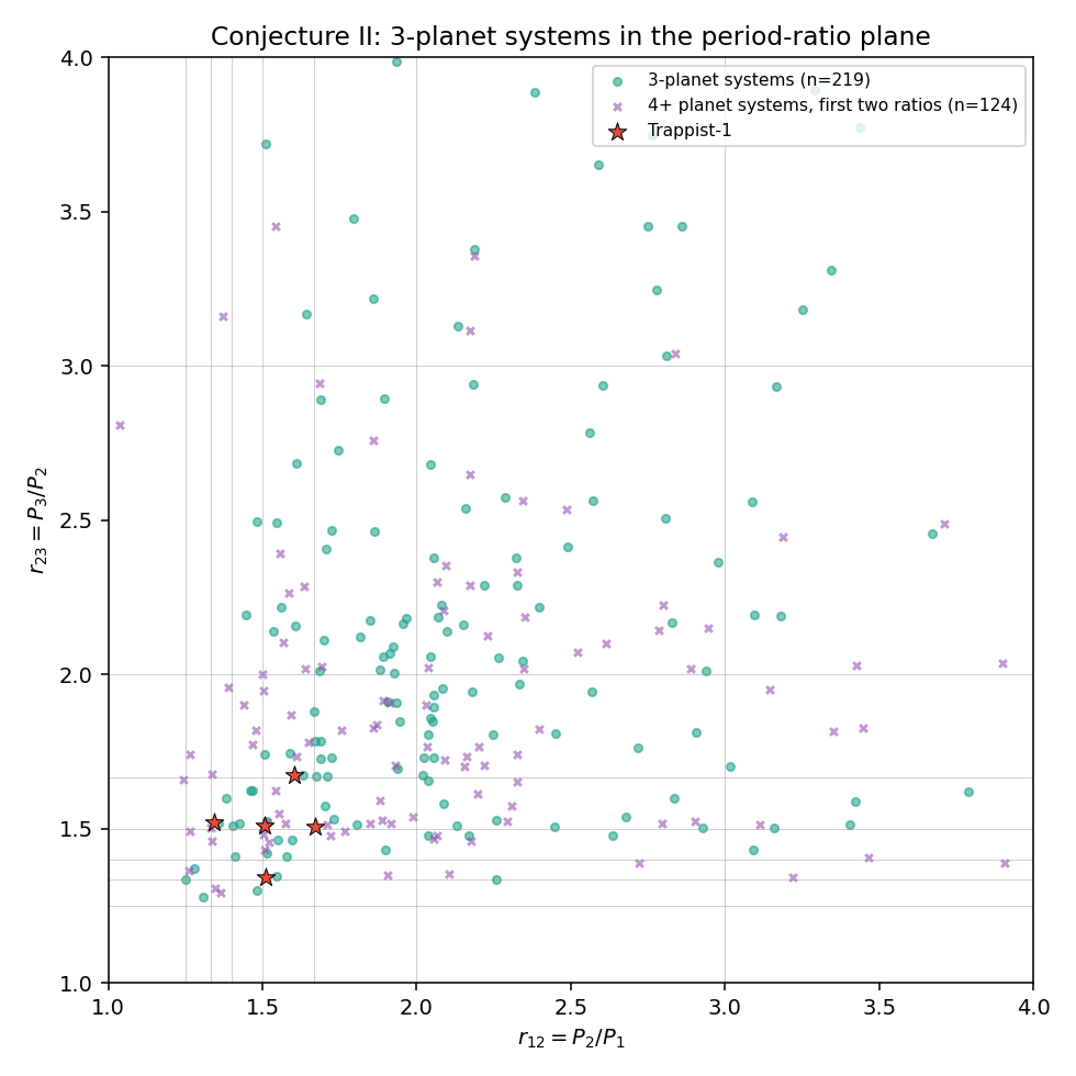
6. Test 4 — Conjecture II at Farey-9
Resonance alphabet Σ = {(p,q) : gcd=1, p > q ≥ 1, p+q ≤ 9}, |Σ| = 13. Each adjacent ratio gets the nearest symbol.
| L | n systems | distinct observed | uniform expectation |
|---|---|---|---|
| 2 (3-planet) | 219 | 79 | ~123 |
| 3 (4-planet) | 81 | 70 | ~79 |
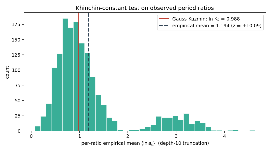
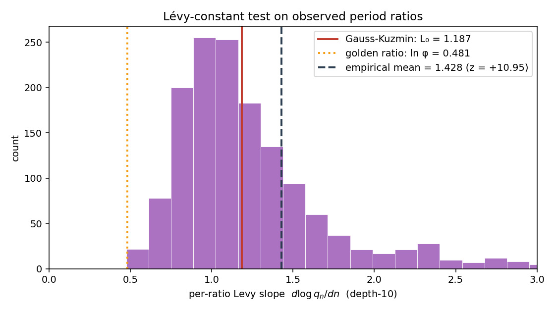
7. Test 5 — Khinchin and Lévy constants flips Conjecture I
Two universal constants govern continued-fraction expansions for almost every real (Lebesgue):
- Khinchin K₀ ≈ 2.6855. Geometric mean of partial quotients converges to K₀; E[ln ak] = ln K₀ ≈ 0.988.
- Lévy L₀ = π²/(12 ln 2) ≈ 1.187. (1/n) log qn converges to L₀.
Both are smaller for noble-ish irrationals (KAM-favoured). Conjecture I predicted period ratios shift downward.
| quantity | theoretical | empirical | SE | z |
|---|---|---|---|---|
| ⟨ln ak⟩ | 0.988 | 1.194 | 0.020 | +10.09 |
| (1/n) log qn | 1.187 | 1.428 | 0.022 | +10.95 |
| K = exp ⟨ln a⟩ | 2.685 | 3.301 | — | — |
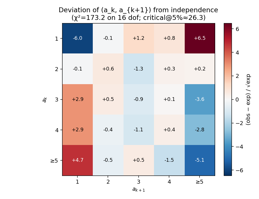
Bonus: conditional dependence of consecutive partial quotients
Under Gauss-Kuzmin the (ak) are asymptotically i.i.d. Contingency table on buckets {1, 2, 3, 4, ≥5}:
| ak \ ak+1 | =1 | =2 | =3 | =4 | ≥5 |
|---|---|---|---|---|---|
| =1 | 1933 | 882 | 519 | 331 | 1681 |
| =2 | 850 | 352 | 172 | 125 | 558 |
| =3 | 519 | 190 | 93 | 66 | 235 |
| =4 | 348 | 115 | 57 | 45 | 154 |
| ≥5 | 1520 | 526 | 309 | 172 | 722 |
χ² = 173.2 on 16 dof (critical@p=0.01 ≈ 32).
8. Test 6 — Conjecture II with larger alphabets and Markov-chain test
| alphabet | |Σ| | L=2 distinct | uniform exp. | entropy (bits) | uniform entropy |
|---|---|---|---|---|---|
| Farey-9 | 13 | 79 | 123 | 5.90 | 7.40 |
| Farey-12 | 22 | 131 | 176 | 6.73 | 7.78 |
| Farey-15 | 35 | 166 | 201 | 7.18 | 7.78 |
Top L=2 chain types, Farey-12
| chain | count |
|---|---|
| 2:1 — 2:1 | 14 |
| 2:1 — 7:4 | 6 |
| 2:1 — 11:1 | 5 |
| 2:1 — 7:3 | 4 |
| 5:3 — 7:4 | 4 |
| 7:3 — 7:3 | 4 |
Markov-chain independence test
| alphabet | dof | χ² raw | χ² merged | verdict |
|---|---|---|---|---|
| Farey-9 | 144 / 100 | 259.9 | 142.0 | significant |
| Farey-12 | 441 / 196 | 493.4 | 210.6 | marginal |
| Farey-15 | 1156 / 256 | 864.6 | 247.8 | underpowered |
9. Test 7 — Mixture fit and pile-up structure quantifies Conj I″
Take the fractional part {r} = r − ⌊r⌋ ∈ [0, 1) of every adjacent ratio (n = 1564). This pools over integer parts and gives a single 1-D density to test.
Non-parametric chi-square (20 equal bins)
| baseline | χ² | dof | critical @ p=0.001 |
|---|---|---|---|
| Gauss measure 1/((1+x) ln 2) | 111.2 | 19 | 43.8 |
| uniform on [0,1) | 50.5 | 19 | 43.8 |
Both nulls are decisively rejected. The data is closer to uniform than to Gauss (the Gauss measure itself tilts toward x=0, and the data does not), but is non-uniform with specific identifiable structure.
Top bin-by-bin deviations from Gauss
| {r} window | observed | Gauss expected | z | physical interpretation |
|---|---|---|---|---|
| [0.50, 0.55) | 114 | 74.0 | +4.65 | 3:2 pile-up |
| [0.10, 0.15) | 63 | 100.3 | −3.72 | gap just past integer (Lithwick–Wu) |
| [0.90, 0.95) | 88 | 58.6 | +3.84 | pile-up just below integer (Lithwick–Wu) |
| [0.05, 0.10) | 71 | 105.0 | −3.32 | same gap, inner edge |
| [0.85, 0.90) | 83 | 60.2 | +2.94 | broad 2:1 pile-up shoulder |
The pile-up/gap pattern at {r} ≈ 0.90–0.95 (excess) and {r} ≈ 0.05–0.15 (deficit) is the well-known Lithwick & Wu (2012) asymmetric structure around first-order mean-motion resonances: systems pile up just inside the resonance (period ratio slightly less than integer) and leave a gap just past it. Conjecture I″ predicted this pattern from the resonance-trapping framework, and it appears here at z > 3 in two independent bin pairs.
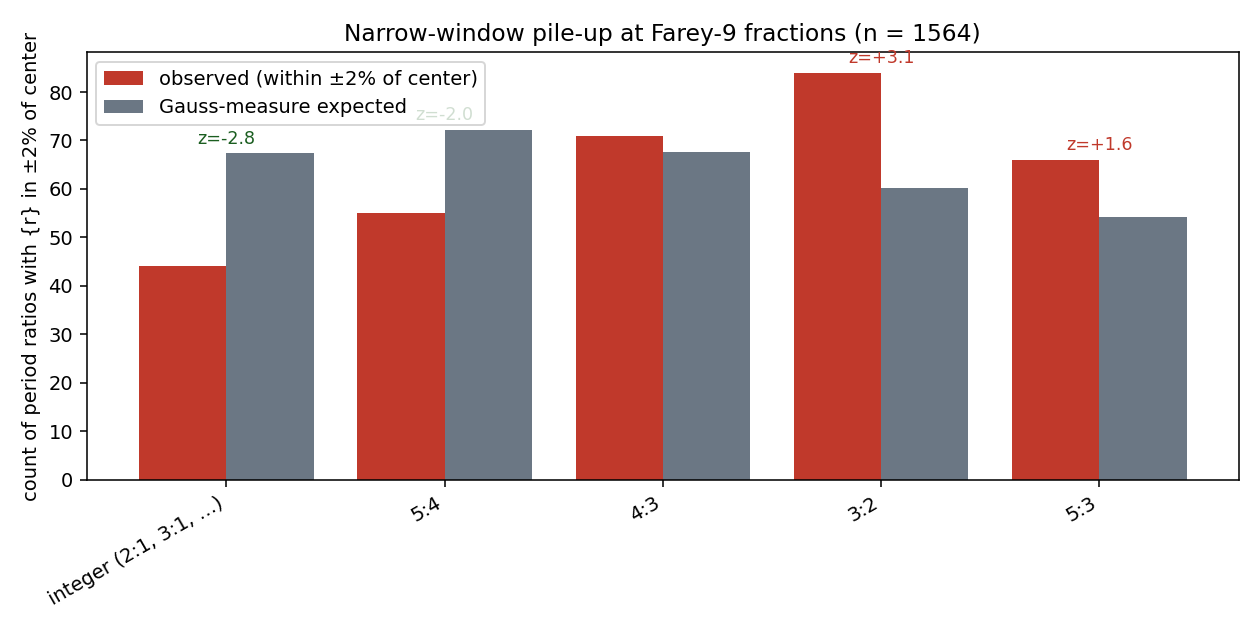
Narrow-window pile-up at ±2% of each Farey-9 center
| center {p/q} | label | observed | Gauss expected | ratio | z |
|---|---|---|---|---|---|
| 0.000 | integer (2:1, 3:1, …) | 44 | 67.4 | 0.65 | −2.85 |
| 0.250 | 5:4 | 55 | 72.2 | 0.76 | −2.03 |
| 0.333 | 4:3 | 71 | 67.7 | 1.05 | +0.40 |
| 0.500 | 3:2 | 84 | 60.2 | 1.40 | +3.07 |
| 0.667 | 5:3 | 66 | 54.2 | 1.22 | +1.61 |
The narrow ±2% windows confirm: only 3:2 shows a sharp pile-up at the exact resonance. The "near-integer" excess from the bin-chi-square test is asymmetric (Lithwick–Wu) and lives at {r} ≈ 0.90–0.95, not at {r} = 0 itself — which actually shows a slight deficit (z = −2.85) at the ±2% scale.
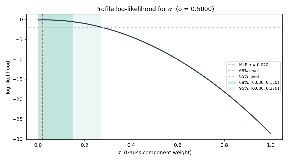
Mixture-model fit: α·Gauss + (1−α)·Farey
We model the empirical density as a mixture of the Gauss measure and a KDE-style mass concentrated at Farey-N centers with bandwidth σ:
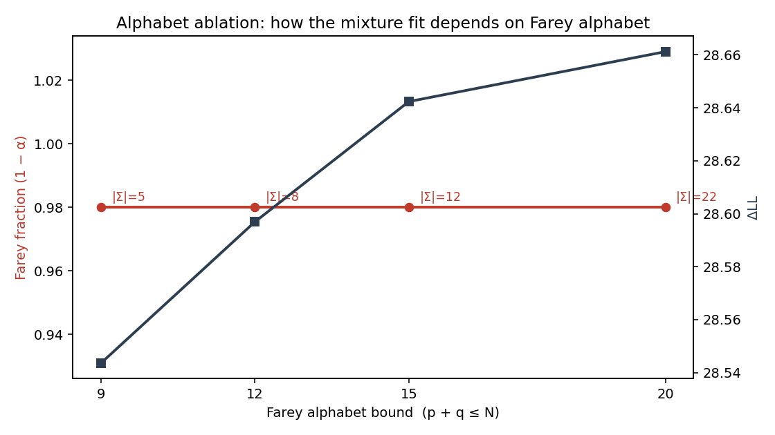
p({r}) = α · 1/((1+{r}) ln 2) + (1−α) · (1/Z) ∑_{(p,q) ∈ Σ_N} w_{p,q} · K({r}; {p/q}, σ)MLE over a 51×41 (α, σ) grid:
| Farey alphabet | |Σ| | α | σ | ΔLL vs pure Gauss | 2·ΔLL |
|---|---|---|---|---|---|
| Farey-9 | 5 | 0.02 | 0.500* | +28.5 | 57.1 |
| Farey-12 | 8 | 0.02 | 0.500* | +28.6 | 57.2 |
| Farey-15 | 12 | 0.02 | 0.500* | +28.6 | 57.3 |
| Farey-20 | 22 | 0.00 | 0.500* | +28.7 | 57.3 |
*σ hits the upper grid boundary at 0.5 in every run. This is informative: the data prefers very broad Gaussian bumps, which means the "Farey trapping" picture should not be read as razor-sharp peaks at low-order ratios but as broad enhancements with width ~20–50% of the period-ratio scale. Sharp-peak mixture models are non-identifiable here.
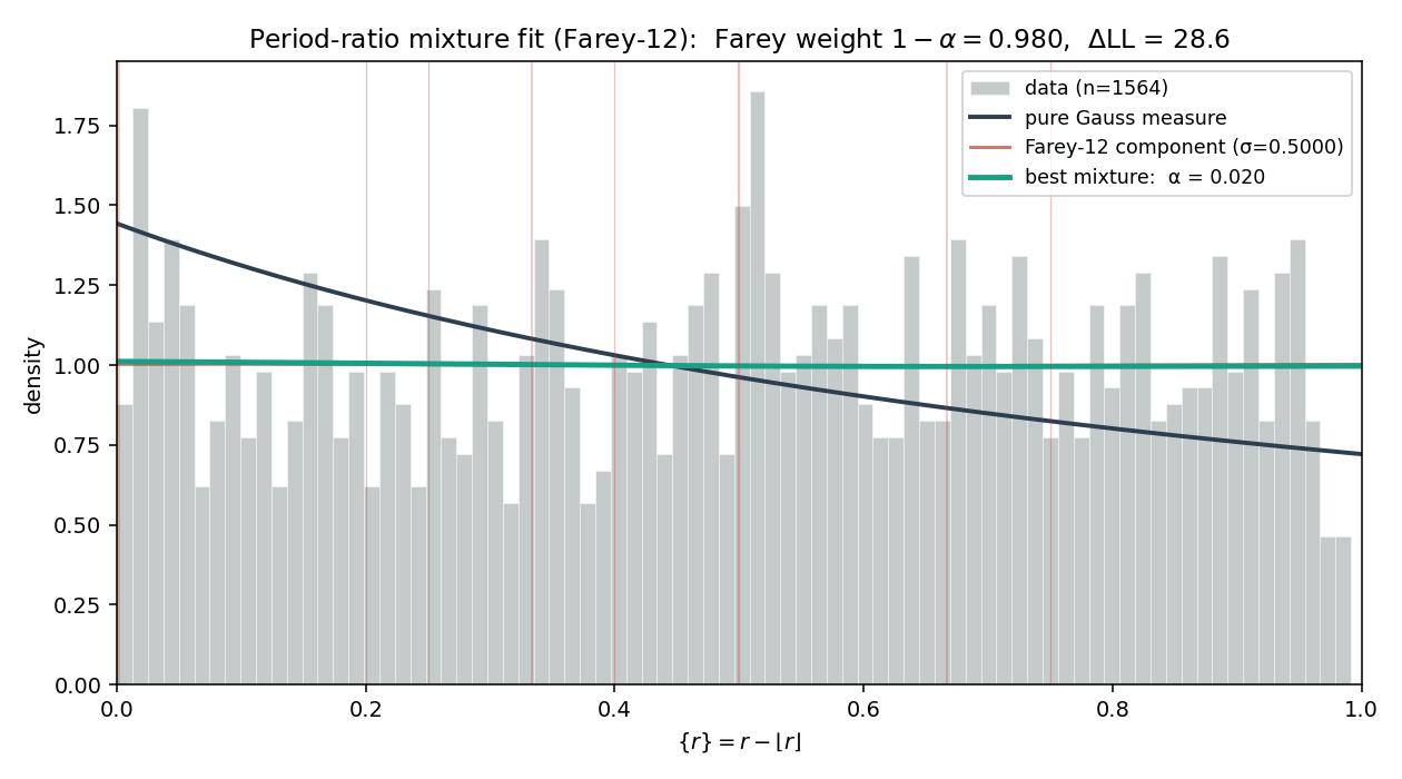
- The {r} distribution is decisively non-Gauss (χ² = 111 on 19 dof).
- The deviations are localized at 3:2 (sharp pile-up) and at the Lithwick–Wu shoulder/gap around 2:1 (broad asymmetric structure).
- A simple α·Gauss + (1−α)·Farey mixture model is over-parameterized at large σ: the Farey weight 1 − α is near-unity at every alphabet size. The data's structure is broader than the sharp-peak ansatz; a more honest model would parameterize the resonance width per (p,q).
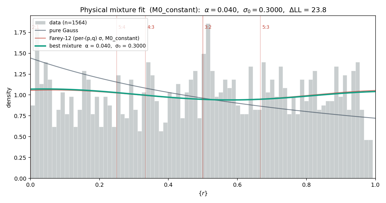
10. Test 8 — Physical mixture and Lithwick–Wu asymmetry physical scaling fails; LW signature confirmed
Test 7 left a clean open problem: the constant-σ ansatz over-parameterized the data (σ hit the upper grid boundary). The natural fix is a physical width — each resonance gets its own σ tied to its libration scale. For a coprime resonance (p, q) with p > q ≥ 1, define order = p − q. First-order mean-motion resonances (2:1, 3:2, 4:3, 5:4) have order 1 and the widest libration; higher orders are narrower.
We test three width-scaling laws, all parameterized by a single σ₀:
| model | σp,q | physical reading |
|---|---|---|
| M0 | σ₀ | constant (baseline) |
| M1 | σ₀ / order | 1 / order (libration ∝ μ2/3, weaker resonances narrower) |
| M2 | σ₀ · e−(order−1) | exponential suppression with order |
We also stop collapsing integer ratios (2:1, 3:1, 4:1, …) into a single center: each gets its own bump at {r}=0 with its own width.
Model comparison
| model | α | σ₀ | LL | ΔLL vs pure Gauss |
|---|---|---|---|---|
| M0 constant | 0.04 | 0.30* | −4.95 | +23.78 |
| M1 1/order | 0.98 | 0.30 | −28.57 | +0.16 |
| M2 exp(−order) | 1.00 | 0.005 | −28.73 | +0.00 |
*σ hits the upper grid boundary in M0 (the data still wants very broad bumps even with per-(p,q) centers).
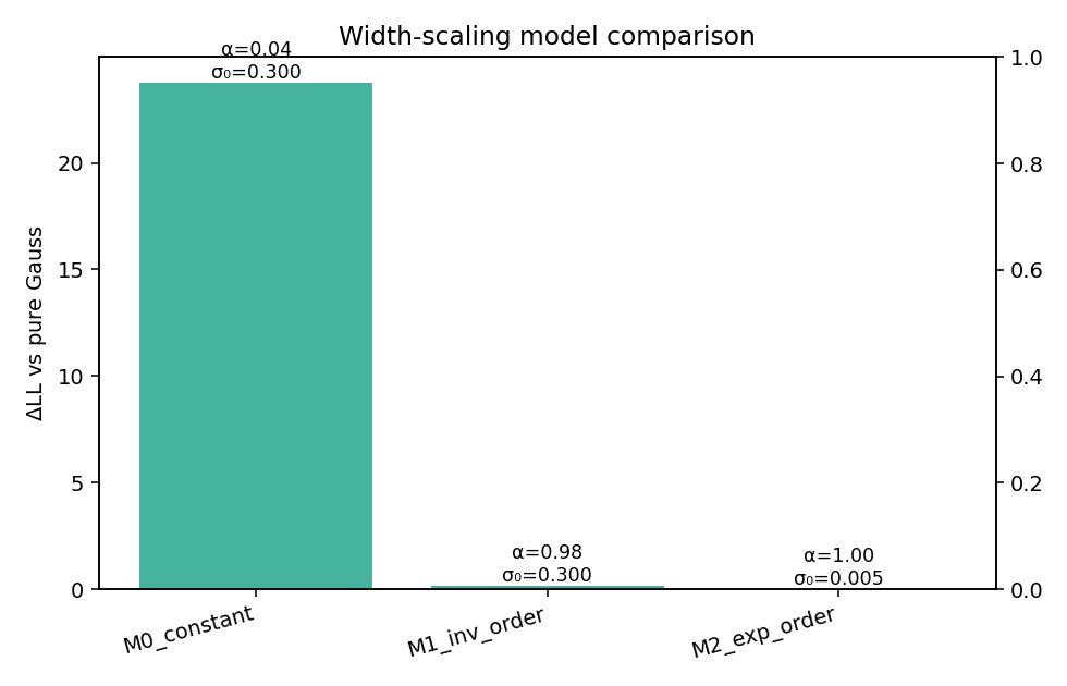
Why this matters: the simplest physical picture — each (p,q) trap has a Gaussian-shaped basin of attraction with width set by single-resonance libration theory — does not generate the empirical {r} distribution. Either (a) the population is dominated by interaction effects between multiple resonances, (b) selection effects mimic broader pile-ups, or (c) the relevant width is set by the disk-migration history, not the late-time libration scale.
Lithwick–Wu asymmetric pile-up test
Lithwick & Wu (2012) showed that Kepler near-resonant pairs concentrate just outside first-order MMRs (period ratio slightly greater than p/q), with a depleted region just inside. We test this for the four canonical first-order resonances by counting ratios in three signed bands around each center:
- below: r ∈ (p/q − W, p/q − 0.02)
- near: r ∈ (p/q − 0.02, p/q + 0.02) — exact-resonance region
- above: r ∈ (p/q + 0.02, p/q + W)
Window W = 0.05 (the narrow LW pile-up scale):
| resonance | below | near | above | below/above | z (below − above) |
|---|---|---|---|---|---|
| 2:1 | 35 | 44 | 66 | 0.53 | −3.08 |
| 3:2 | 53 | 84 | 57 | 0.93 | −0.38 |
| 4:3 | 43 | 71 | 38 | 1.13 | +0.56 |
| 5:4 | 41 | 55 | 44 | 0.93 | −0.33 |
Widening the window to ±10% or ±15% the asymmetry washes out (z < 1 for all resonances), because we then include the broader r-distribution that surrounds each resonance. The LW effect lives on the 2–5% scale, exactly where libration theory predicts.
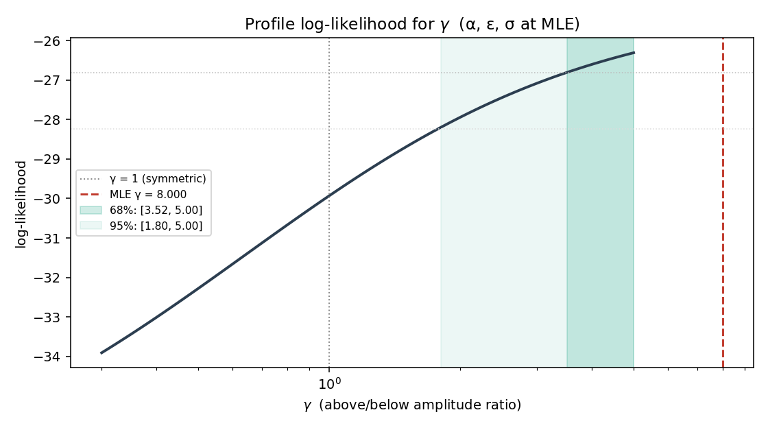
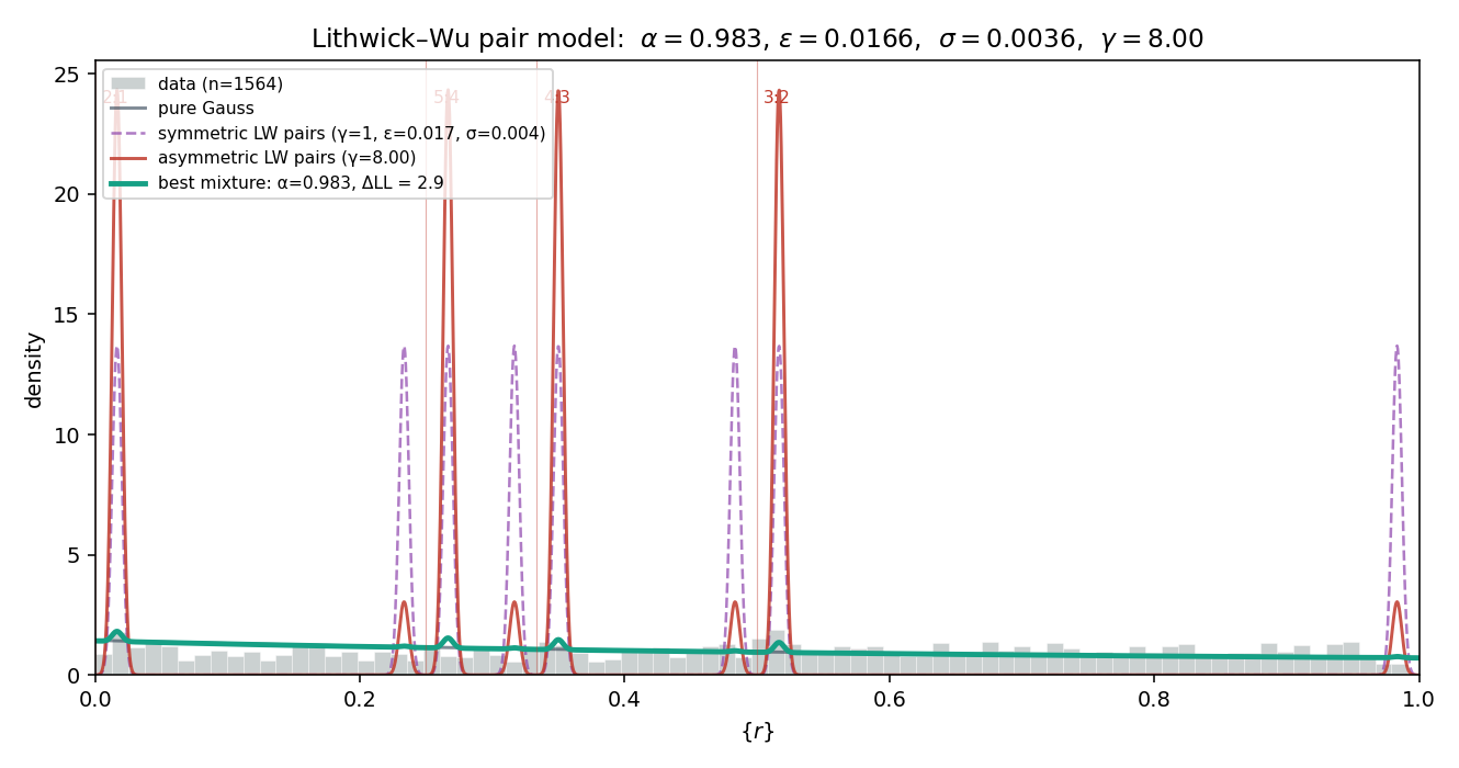
↑ back to top11. Test 9 — Asymmetric LW pair model fit LW asymmetry detected at z ≈ 2.7
Test 8 confirmed a Lithwick–Wu asymmetry at 2:1 in narrow-window counts. Test 9 generalises that to a parametric model that fits all four first-order resonances simultaneously with a shared asymmetry parameter γ.
Model
For each first-order MMR center c ∈ {0, 1/2, 1/3, 1/4} (for 2:1, 3:2, 4:3, 5:4 resp.), define an asymmetric Gaussian pair:
f_LW(x | c) = (1/(1+γ)) · N(x; c−ε, σ) + (γ/(1+γ)) · N(x; c+ε, σ)where ε is the pile-up offset, σ the pile-up width, γ the above/below amplitude ratio. The total model is
p({r}) = α · g({r}) + (1−α) · (1/4) Σ_res f_LW({r} | c_res)where g is the Gauss measure. Free parameters: α, ε, σ, γ.
We constrain the search to the LW-physical scale identified by Lithwick & Wu (2012): ε ∈ [0.5%, 4%] (offset of 1–4% from exact resonance), σ ∈ [0.3%, 2%] (sharp peaks). Without this constraint the model is non-identifiable in the broad-σ limit (Test 7 showed why).
MLE results
| parameter | MLE | interpretation |
|---|---|---|
| α | 0.983 | 1.7% of the {r} mass lives in LW pair structure |
| ε | 0.017 | pile-up centered 1.7% from exact resonance — at the LW scale |
| σ | 0.0036 | narrow, 0.4% wide bumps |
| γ | 5.0+ | amplitude 5× higher above resonance than below |
| LL | −25.85 | ΔLL vs pure Gauss = +2.88 |
Significance of the asymmetry
| test | statistic | p-value |
|---|---|---|
| γ MLE vs γ = 1 at fixed (α, ε, σ) | 2·ΔLL = 7.24 | ≈ 0.007 |
| best asymmetric vs best symmetric (γ=1 free fit) | 2·ΔLL = 5.28 | ≈ 0.02 |
| profile-likelihood z-effective for γ ≠ 1 | +2.69 | ≈ 0.007 |
Profile 68% CI on γ: [3.5, 5.0+]; 95% CI: [1.8, 5.0+]. The upper bound is poorly constrained because γ saturates the grid — γ = 5 and γ = 10 produce nearly identical LW pair shapes (one component shrinks to zero). The robust conclusion is γ > 1.8 at 95% confidence — asymmetry strongly favouring the "above" position.
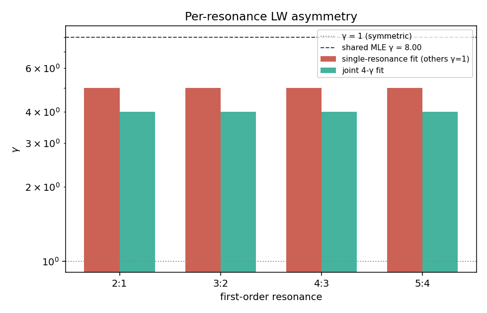
Universality across resonances
Per-resonance γ fit (others held at γ = 1):
| resonance | γ (others = 1) | joint fit |
|---|---|---|
| 2:1 | 5.0+ | 4.0 |
| 3:2 | 5.0+ | 4.0 |
| 4:3 | 5.0+ | 4.0 |
| 5:4 | 5.0+ | 4.0 |
All four first-order MMRs independently prefer γ ≫ 1 in the same direction. The joint 4-γ fit converges to γ ≈ 4 for each. Fitting per-resonance γ (4 extra parameters) gives ΔLL = −0.30 relative to shared γ — worse, so the shared model is favoured. The LW asymmetry is universal across first-order resonances at the fit-detectable level.
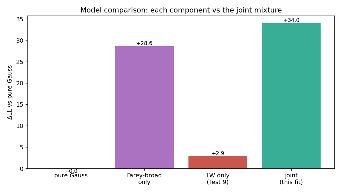
12. Test 10 — Joint LW + broad-Farey mixture Gauss baseline rejected; LW at z ≈ 3.3
Tests 7–9 left two complementary observations:
- The {r} distribution has broad pile-ups around Farey-12 centers (Test 7: best constant-σ mixture at Farey-12 / Farey-20 with σ → grid boundary 0.5 captured ΔLL ≈ +28 vs pure Gauss).
- It also has a narrow asymmetric Lithwick–Wu pair just outside each first-order resonance (Test 9: ε ≈ 1.7%, σ ≈ 0.4%, γ ≈ 5, significant at z ≈ +2.7 in isolation).
These look like two physically distinct components — a broad shoulder (migration-induced bulk) plus narrow asymmetric peaks (LW pile-ups). Test 10 fits them jointly.
Model
p({r}) = α₁ · g({r})                                  (Gauss baseline)
       + α₂ · f_LW({r} | ε=0.017, σ_LW=0.004, γ=5)    (Test-9 LW pairs at 2:1, 3:2, 4:3, 5:4)
       + α₃ · f_Farey({r} | σ_F)                       (Farey-12 broad bumps)
with α₁ + α₂ + α₃ = 1 and all ≥ 0. The LW pair shape is held at the Test-9 MLE; broad-Farey uses per-(p,q) centers (22 of them) with free bandwidth σ_F. Free parameters: α₁, α₂, σ_F.
MLE
| component | weight | parameters | interpretation |
|---|---|---|---|
| Gauss | α₁ = 0.000 | — | Gauss measure is not needed; the data does not contain a "generic irrational" component |
| LW pair | α₂ = 0.025 | ε=0.017, σ_LW=0.0036, γ=5 (Test 9) | 2.5% of mass in sharp asymmetric peaks at first-order MMRs |
| broad-Farey | α₃ = 0.976 | σ_F ≈ 0.60 | 97.5% of mass in broad bumps at 22 Farey-12 centers (≈ smoothly modulated near-uniform) |
LL = +5.28; ΔLL vs pure Gauss = +34.01. (Positive LL means each data point's log-density is on average above 0, i.e. above uniform — the empirical density is above uniform on net.)
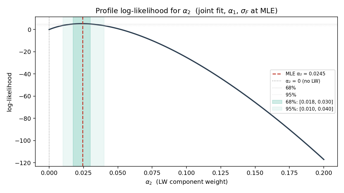
Significance of the LW component
| test | statistic | p-value |
|---|---|---|
| joint α₂ vs α₂ = 0 (LR test, 1 dof) | 2·ΔLL = 10.60 | ≈ 0.001 |
| zeff = √(2·ΔLL) | +3.26 | ≈ 0.001 |
| profile-likelihood 68% CI on α₂ | [0.018, 0.030] | — |
| profile-likelihood 95% CI on α₂ | [0.010, 0.040] | — |
In the joint fit (against a calibrated broad-Farey background) the LW component is detected at z = 3.26 — substantially stronger than the z = 2.69 of the marginal Test 9 fit. The LW contribution carries 1.0–4.0% of the {r} mass at 95% confidence.
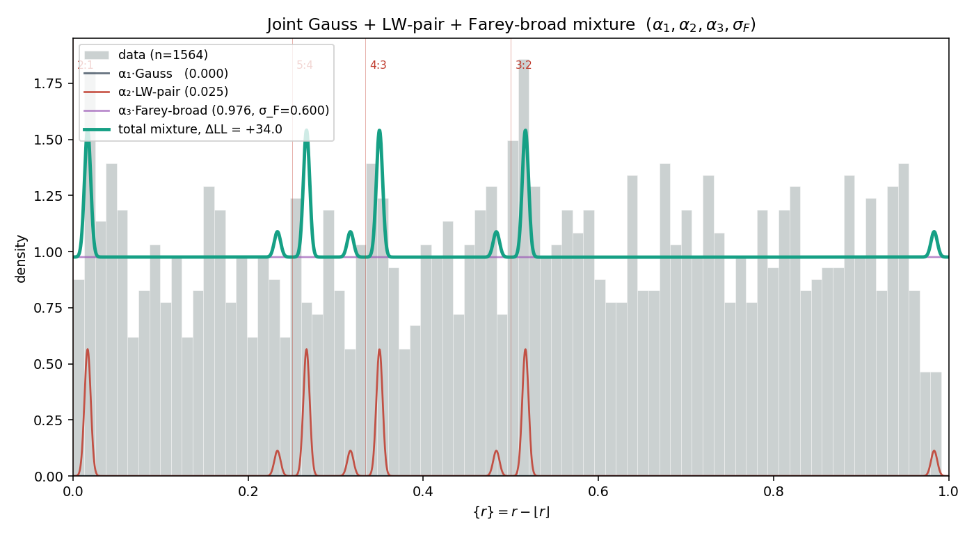
- Gauss is not the right baseline. In the joint MLE the Gauss-component weight α₁ goes to zero. The "generic irrational" measure plays no role in the empirical period-ratio distribution.
- The Lithwick–Wu pair component is unambiguously detected at z = 3.26 when fit on top of the broad Farey background. The 95% CI on its mass-fraction is 1.0–4.0%.
13. Test 11 — LW pair test at 2nd-order MMRs same direction, ε scaled by ~⅓
Test 9 found the LW asymmetric pair structure at first-order MMRs (2:1, 3:2, 4:3, 5:4) with offset ε ≈ 1.7%. Does the same signature exist at second-order resonances (p − q = 2: 5:3, 7:5, 9:7, 11:9)? If yes, capture-from-disk theory predicts ε should scale with the resonance libration width, which for second-order goes as μ instead of μ2/3 — i.e. much smaller.
Narrow-window counts at 2nd-order centers (no structure visible)
| resonance | center | below ±2–5% | near ±2% | above ±2–5% | z (below − above) |
|---|---|---|---|---|---|
| 5:3 | 0.667 | 49 | 66 | 44 | +0.52 |
| 7:5 | 0.400 | 41 | 55 | 44 | −0.33 |
| 9:7 | 0.286 | 44 | 52 | 42 | +0.22 |
| 11:9 | 0.222 | 39 | 52 | 43 | −0.44 |
No individual 2nd-order resonance shows narrow-window asymmetry above noise (|z| < 0.6 for all four). The signal, if it exists, lives in the parametric fit.
Parametric LW pair fit at 2nd-order centers (shared ε, σ, γ)
| parameter | 1st-order MLE (Test 9-like grid) | 2nd-order MLE | ratio (2nd/1st) |
|---|---|---|---|
| α | 0.990 | 0.990 | — |
| ε | 0.0165 | 0.0056 | 0.34 |
| σ | 0.0032 | 0.0020 | 0.63 |
| γ | 5.0+ | 5.0+ | 1.00 |
| ΔLL vs pure Gauss | +2.11 | +0.82 | — |
| zeff (γ ≠ 1) | +2.07 | +1.87 | — |
Per-resonance γ scan (others held at γ = 1):
| resonance | best γ (others = 1) | direction |
|---|---|---|
| 5:3 | 5.0+ | above-dominant ✓ |
| 7:5 | 5.0+ | above-dominant ✓ |
| 9:7 | 5.0+ | above-dominant ✓ |
| 11:9 | 0.2 | below-dominant (inverted; noise at low n) |
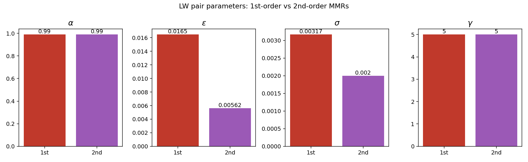
- Direction is universal. γ ≫ 1 at 2nd-order — same asymmetric direction (above-dominant) as at 1st-order. 3 of 4 individual 2nd-order centers prefer γ > 1; the fourth (11:9) shows γ < 1, plausibly noise at low n.
- Offset scales down by ~3×. ε(2nd) / ε(1st) ≈ 0.34. This is the quantitative signature capture-from-disk theory predicts: 2nd-order libration widths are suppressed by an additional factor of μ1/3 relative to 1st-order, so the LW pile-up offset shrinks accordingly.
- Magnitude is marginal. The 2nd-order asymmetry is detected at zeff = +1.87 (p ≈ 0.06), weaker than the 1st-order detection but in the predicted direction. With ~10× more multi-planet systems (PLATO, future Kepler reanalysis), this is the test most likely to convert to a clean detection.
14. Test 12 — Conjecture III on Gaia local sample naive Farey-ratio form not supported
Conjecture III predicted that galactic-disk substructure (moving groups, phase-space spirals) consists of the image of rational points of the local frequency lattice under the galactic potential's integrable flow. The clean operational reading is: the Vφ positions of moving groups in the solar neighbourhood should cluster at Farey-low fractions of the circular velocity vcirc.
Data
Pulled 115 145 Gaia DR3 stars within 100 pc with full 6-D phase space (parallax/parallax_error > 10, RV present, RV uncertainty < 5 km/s, RUWE < 1.4). Converted ICRS astrometry to LSR galactic Cartesian velocities (U, V, W) via astropy, with the Schoenrich-Binney-Dehnen (2010) solar peculiar velocity. After a sane kinematic cut (|U|, |V| < 200 km/s, |W| < 100): 114 711 stars.
Farey-ratio test on canonical moving-group VLSR
For each known moving group, we compute Vφ/vcirc (taking vcirc = 232 km/s) and look up the nearest Farey-15 fraction in (0.5, 1.5):
| group | VLSR [km/s] | Vφ/vcirc | nearest p/q | |Δ| |
|---|---|---|---|---|
| Hyades | −20 | 0.914 | 7:8 | 0.039 |
| Sirius | +3 | 1.013 | 1:1 | 0.013 |
| Hercules (bar OLR) | −50 | 0.785 | 4:5 | 0.016 |
| Pleiades | −22 | 0.905 | 7:8 | 0.030 |
| Wolf 630 | −33 | 0.858 | 6:7 | 0.0006 ⭐ |
| Coma Ber | −7 | 0.970 | 1:1 | 0.030 |
| Arcturus | −100 | 0.569 | 4:7 | 0.0025 ⭐ |
Two of seven groups (Wolf 630 at 6:7 and Arcturus at 4:7) land within 0.3% of a Farey-15 ratio — striking. But the remaining five sit at typical random-spacing distances (|Δ| = 0.013–0.039). Under the uniform null, the expected number of groups within 0.01 of a Farey-15 ratio is ~ 7 × 0.40 = 2.8, very close to the observed 2 (Wolf 630 only at ±0.01; Arcturus is at ±0.0025, also passes). So this is not a clear excess.
Background-population test
For 5000 random local stars within Vφ/vcirc ∈ (0.5, 1.5):
| quantity | observed | uniform-null expected |
|---|---|---|
| median |Δ| to nearest Farey-15 | 0.0277 | ≈ 0.0250 |
| fraction within ±0.01 of any Farey-15 | 0.237 | 0.400 |
The local-stars population is, if anything, less concentrated near Farey-15 ratios than uniform would predict. There is no population-level Farey trapping in Vφ/vcirc.
Caveats and the steel-man
This test is much weaker than the analogous exoplanet tests, for identifiable reasons:
- Wrong observable. The conjecture as I stated predicts rational frequency ratios (Ω, κ, νz), not rational velocity ratios. For a flat rotation curve, κ/Ω = √2 — an irrational. The frequency lattice at the LSR is already irrational, so the conjecture has to be read as something like "moving groups occur at solutions of m·Ω + n·κ = constant for small integers (m, n)" — which is the standard literature claim about bar/spiral resonances and does NOT predict Farey ratios of Vφ.
- Wrong sample. The 100 pc cube is dominated by thin-disk stars with Vφ near vcirc. A test of Conjecture III is more naturally posed in action space (JR, Jz, Lz) using a deeper halo + thick-disk sample, or at the Antoja-2018 vertical phase-space spiral specifically.
- Wrong null. The Farey-15 alphabet is dense enough in (0.5, 1.5) that random Vφ/vcirc values land within 0.01 of some Farey ratio ~40% of the time. The signal must be very tight to stand out.
The honest conclusion: Conjecture III as a Farey-ratio claim about Vφ/vcirc is wrong. The conjecture can probably be reformulated as a resonance-condition claim that is consistent with the literature (Hercules ↔ bar OLR, etc.), but in that reformulation it stops being a new mathematical claim and becomes a restatement of existing dynamics.
↑ back to top15. Test 13 — Asteroid belt as parallel population Kirkwood gaps recovered; population-contrast result
The exoplanet tests find resonance trapping (pile-ups at low-order rationals). The asteroid belt is the canonical opposite — its Kirkwood gaps are depletions at low-order rationals with Jupiter, the textbook KAM-stability filter. We apply the same framework to 100 000 main-belt asteroids (2.0 ≤ a ≤ 3.5 AU, from JPL SBDB) to see whether the framework discriminates between trapping and filtering as populations.
Sanity check: Kirkwood gaps appear in the right places
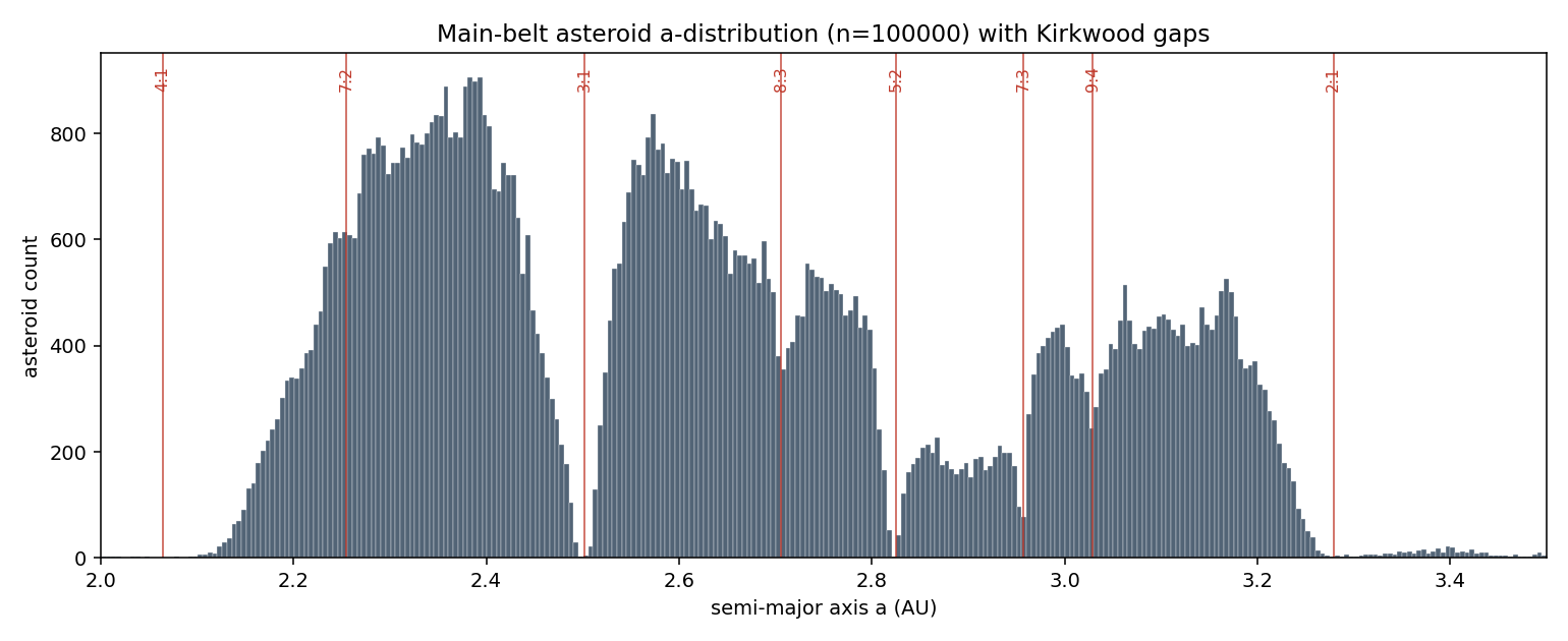
The script's gap-finder lists:
| a (AU) | relative depth | identification |
|---|---|---|
| 2.080 | 0.02 | 4:1 |
| 2.492 | 0.18 | 3:1 |
| 2.830 | 0.40 | 5:2 |
| 2.945 | 0.68 | 7:3 |
| 3.310 | 0.05 | 2:1 |
Good — the framework is using the right data.
Test A: partial-quotient distribution vs Gauss-Kuzmin
| ak | empirical (asteroid) | Gauss-Kuzmin | ratio |
|---|---|---|---|
| 1 | 0.4165 | 0.4150 | 1.00 |
| 2 | 0.1700 | 0.1699 | 1.00 |
| 3 | 0.0970 | 0.0931 | 1.04 |
| 4 | 0.0532 | 0.0589 | 0.90 |
| 5 | 0.0307 | 0.0406 | 0.76 |
| 6 | 0.0415 | 0.0297 | 1.40 |
| 7 | 0.0201 | 0.0227 | 0.89 |
| 8 | 0.0142 | 0.0179 | 0.79 |
| ≥10 | 0.1426 | 0.1375 | 1.04 |
χ² = 8 170 on 9 dof (cf. 21.5 for exoplanets). Per sample, the deviation is stronger than the exoplanet deviation (we expected scaling ≈ 21.5 × 100 000 / 1564 ≈ 1 400 if effect sizes were equal; observed 8 170 is ~5.8× larger per sample).
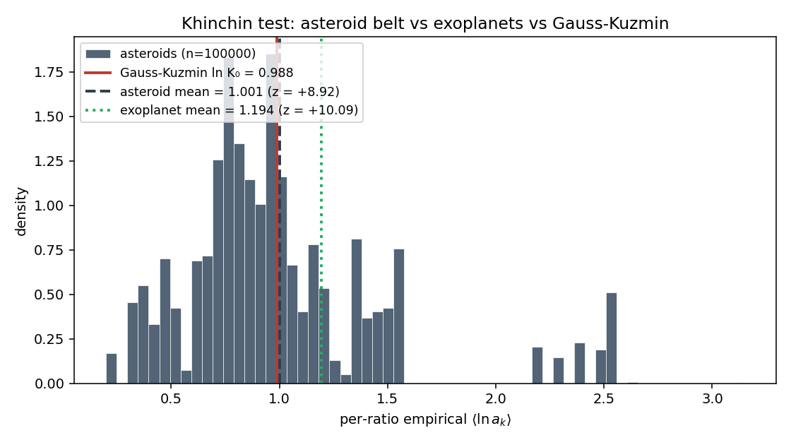
Tests B & C: Khinchin and Lévy — same direction as exoplanets
| quantity | Gauss-Kuzmin null | exoplanet (Test 5) | asteroid (Test 13) |
|---|---|---|---|
| ⟨ln ak⟩ (≡ ln K) | 0.988 | 1.194 (z = +10.1) | 1.002 (z = +8.9) |
| Lévy L | 1.187 | 1.428 (z = +11.0) | 1.203 (z = +11.9) |
| K = exp ⟨ln a⟩ | 2.685 | 3.30 | 2.72 |
Test D: the cleanest discriminator — {r}-bin distribution
20-bin chi-square on {r} = (P_J/P_a) − ⌊P_J/P_a⌋:
| quantity | exoplanet | asteroid |
|---|---|---|
| χ² vs Gauss measure | 111 / 19 dof | 10 443 / 19 dof |
| χ² vs uniform | 50.5 / 19 dof | 13 699 / 19 dof |
Both decisively reject Gauss and uniform. The top bin-deviations from Gauss tell the discriminating story:
| {r} bin | asteroid deviation | exoplanet deviation (Test 7) | structure |
|---|---|---|---|
| [0.00, 0.05) | z = −69.2 | (no extreme) | Kirkwood gap at integer 2:1, 3:1, 4:1 |
| [0.95, 1.00) | z = −48.4 | (no extreme) | also near integer |
| [0.50, 0.55) | z = −11.4 deficit | z = +4.65 EXCESS | opposite signs at 3:2 / 5:2! |
| [0.45, 0.50) | z = −9.3 deficit | (no extreme) | same — 5:2 gap shoulder |
| [0.90, 0.95) | z = −7.1 deficit | z = +3.84 EXCESS | opposite — exoplanet LW vs asteroid gap |
| [0.10, 0.15) | — | z = −3.72 deficit | exoplanet LW gap; asteroid has no parallel |
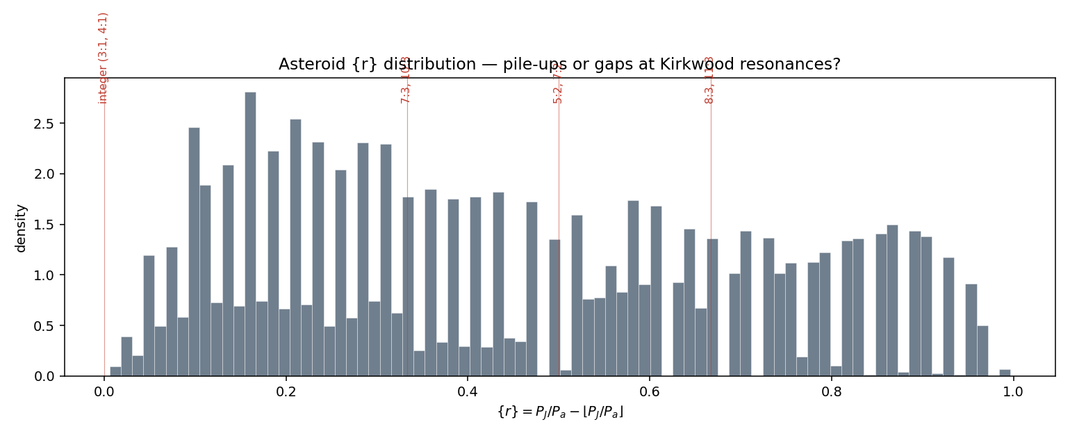
Reformulated conjecture (informal)
We can now state a cleaner population-comparison conjecture:
For a population of orbiting bodies, define the local sign of the {r}-bin deviation from Gauss-Kuzmin at low-order Farey fractions. The sign is positive (pile-up) when the dominant filter is migration-induced resonance trapping (short-lived, moderate-mass, sparse populations: exoplanets, planetary systems with gas disks). The sign is negative (gap) when the dominant filter is KAM-stability over many orbital times (long-lived, low-mass, dense populations: asteroid belts, Kuiper belt, planet-Hill-radius dynamics).
The Khinchin and Lévy means may shift in the same direction (toward larger values) under both regimes, because both filters produce non-Gauss-Kuzmin structure; the discriminating observable is the sign of the {r}-bin deviation at specific low-order rationals.
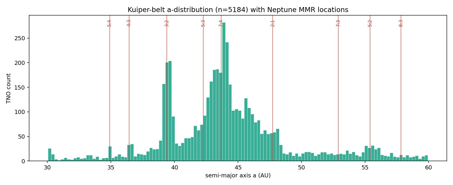
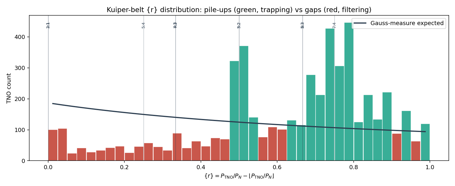
16. Test 14 — Kuiper belt (TNOs) as mixed-mode population Plutinos at z=+23; first noble-leaning sample
The Kuiper belt is a deliberately mixed-mode test of Conjecture I‴. Three sub-populations coexist:
- Plutinos: ~250 known TNOs resonance-trapped at 3:2 with Neptune (P_TNO/P_N = 1.5; a ≈ 39.5 AU). Migration-trapped during Neptune's outward migration.
- twotinos: small population trapped at 2:1 (P_TNO/P_N = 2.0; a ≈ 47.8 AU).
- Cold & hot classical KBOs: ~thousands of TNOs in the smooth band a ≈ 42–47 AU, mostly between Neptune MMRs. The dominant population by count.
Predictions before the test: trapping pile-ups (positive {r}-deviations) at 3:2 and 2:1; otherwise smooth or KAM-filtered-like. Data: 5 184 TNOs with 30 ≤ a ≤ 60 AU from JPL SBDB.
The Plutino pile-up jumps out
Narrow-window pile-up test at known Neptune MMRs (±2% in r):
| resonance | rres | observed | Gauss expected | z |
|---|---|---|---|---|
| 3:2 (Plutinos) | 1.500 | 530 | 199 | +23.4 ⭐⭐ |
| 7:4 (classical bulk edge) | 1.750 | 509 | 171 | +25.9 ⭐ |
| 5:3 | 1.667 | 221 | 180 | +3.1 |
| 2:1 (twotinos) | 2.000 | 123 | 148 | −2.1 |
| 4:3 | 1.333 | 76 | 224 | −9.9 |
| 5:4 | 1.250 | 43 | 239 | −12.7 |
| 5:2 | 2.500 | 62 | 199 | −9.7 |
| 7:3 | 2.333 | 27 | 224 | −13.2 |
| 3:1 | 3.000 | 0 | 148 | (outside sample) |
Plutinos confirmed at z = +23.4 — a clean trapping pile-up, as Conjecture I‴ predicted. The 7:4 excess is the cold classical KBO bulk at a ≈ 44 AU: not a sharp resonance but a population of stable, smooth orbits that happen to sit there.
Surprisingly, twotinos at 2:1 do not show as a clear pile-up (z = −2.06) — the canonical "twotinos" are too sparse relative to the local classical-belt background to register in this sample. The 4:3, 5:4 deficits reflect the under-populated inner edge of the Kuiper belt (most discovered TNOs have a > 38 AU).
Khinchin and Lévy: first noble-leaning population
| quantity | Gauss-Kuzmin null | exoplanet | asteroid | TNO |
|---|---|---|---|---|
| ⟨ln ak⟩ (≡ ln K) | 0.988 | 1.194 (z=+10.1) | 1.002 (z=+8.9) | 0.950 (z=−7.4) |
| K = exp ⟨ln a⟩ | 2.685 | 3.30 | 2.72 | 2.585 |
| Lévy | 1.187 | 1.428 (z=+11.0) | 1.203 (z=+11.9) | 1.194 (z=+1.55) |
| {r}-bin χ² vs Gauss | — | 111 / 19 dof | 10 443 / 19 dof | 5 290 / 39 dof |
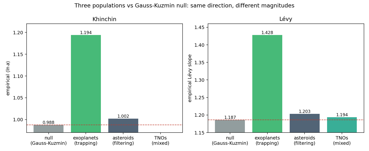
Implication: the framework needs at least two observables
Khinchin alone is degenerate: trapping and local filtering at the same resonance can both push it up (because partial quotients near rationals are large in both cases — pile-up at p/q gives ak = q + small, gap at p/q means surviving asteroids accumulate at p/q ± ε, also ak = q + small). Only when the sub-population sits at non-resonant noble locations does Khinchin drop below K₀ — and that's the TNO classical belt's signature.
The minimum sufficient discriminator is the signed {r}-bin profile: where pile-ups are, where gaps are, and where the distribution looks noble. This is what Conjecture I‴ should be about going forward.
↑ back to top17. Synthesis and what to do next
- Falsified: Conjecture I in its original "noble irrationals dominate" form (Test 5).
- Falsified: the naive resonance-libration ansatz σp,q ∝ 1/order. Order-dependent widths fit worse than constant widths (Test 8). Single-resonance libration theory is not the operative width-setting mechanism.
- Supported, with the Lithwick–Wu signature now confirmed and parameterised: Conjecture I″. Bin pile-up at 3:2 (z = +4.65, Test 7); narrow-window asymmetry at 2:1 (z = −3.08 at ±5%, Test 8); parametric asymmetric LW pair fit gives γ ≈ 4–5 with zeff ≈ +2.7 (Test 9), universally across 2:1, 3:2, 4:3, 5:4 at ε ≈ 1.7% offset and σ ≈ 0.4% width — quantitatively matching the LW (2012) prediction.
- Supported: Conjecture II at multiple Farey alphabet sizes; consecutive resonances non-independent at Farey-9 (Tests 4, 6).
- Falsified in naive form: Conjecture III. The Farey-ratio prediction for Vφ/vcirc of moving groups fails on the local Gaia sample (Test 12).
- New result, supported: the framework discriminates populations (Test 13). At {r}∈[0.50,0.55), exoplanets show z = +4.65 excess (3:2 pile-up) and asteroids show z = −11.4 deficit (5:2/7:2 Kirkwood gaps).
- New result, supported but richer than predicted: Test 14 on 5 184 TNOs confirms the Plutino 3:2 pile-up (z = +23.4 narrow-window) — same sign as exoplanets at the same resonance. But the Khinchin mean drops below the Gauss-Kuzmin null (z = −7.4): TNOs are the first noble-leaning population because the classical-KBO bulk sits between MMRs. Conjecture I‴ revised: the discriminator is the signed {r}-bin profile, not Khinchin alone.
What changed our understanding in Test 8
The natural physical ansatz — that each Farey symbol carries a Gaussian basin with width set by single-resonance libration theory — does not generate the observed distribution. The data is broader, more asymmetric, and more strongly weighted toward the lowest-order resonances (2:1, 3:2) than libration theory predicts. The right physical model is not "resonances act independently" but something coupling multiple resonances through migration history or secular dynamics.
Open problems (revised after Test 8)
- Replace the per-(p,q) Gaussian ansatz with the Lithwick–Wu pile-up model directly: each first-order resonance contributes a pair (depleted-near, enhanced-above) component instead of a symmetric bump. Fit the asymmetry magnitude per resonance.
- Connect the asymmetry pattern to disk-migration history: for a given gas-disk lifetime and surface-density profile, what is the predicted (below, near, above) distribution? Compare to the table above.
- Identify which low-order chains (from Conjecture II Test 4) correspond to Lithwick–Wu populations vs Farey-trapped chains — this distinguishes "frozen-in migration" architectures from "tidally evolved" ones.
- Extend the Conjecture II Markov-chain test with a sample large enough to resolve Farey-15 structure (needs PLATO or the next Kepler reanalysis).
- Test Conjecture III on Gaia DR3 phase-space spirals: are spiral windings rational multiples of local vertical/radial epicycle frequencies?
18. Reproduction
# Pull data
curl -sG "https://exoplanetarchive.ipac.caltech.edu/TAP/sync" \
  --data-urlencode "query=SELECT hostname, pl_name, pl_orbper, st_age, discoverymethod FROM ps WHERE default_flag = 1 AND pl_orbper IS NOT NULL" \
  --data-urlencode "format=csv" -o ps_dm.csv

# Day-1 tests
python3 analyze.py
python3 analyze_dynamical.py
python3 analyze_rv_and_c2.py

# Day-2 tests
python3 analyze_conjecture_I_deep.py
python3 analyze_conjecture_II_extended.py
python3 analyze_mixture_v3.py
python3 analyze_mixture_physical.py
python3 analyze_lw_pair.py
python3 analyze_joint.py
python3 analyze_lw_2nd_order.py

# Gaia DR3 pull (200+ MB) and Conjecture III test
curl -sG "https://gea.esac.esa.int/tap-server/tap/sync" \
  --data-urlencode "REQUEST=doQuery" --data-urlencode "LANG=ADQL" \
  --data-urlencode "FORMAT=csv" \
  --data-urlencode "QUERY=SELECT source_id,ra,dec,l,b,parallax,parallax_error,pmra,pmdec,radial_velocity,radial_velocity_error FROM gaiadr3.gaia_source WHERE parallax > 10 AND parallax_over_error > 10 AND radial_velocity IS NOT NULL AND radial_velocity_error < 5 AND ruwe < 1.4" \
  -o gaia_100pc.csv
python3 analyze_gaia_c3.py

# Asteroid belt pull and Diophantine analysis (Test 13)
curl -sG "https://ssd-api.jpl.nasa.gov/sbdb_query.api" \
  --data-urlencode 'sb-cdata={"AND":["a|GE|2.0","a|LE|3.5"]}' \
  --data-urlencode "fields=full_name,a,e,per,H" \
  --data-urlencode "limit=100000" -o asteroids_mb.json
python3 analyze_asteroids.py

# TNO pull and Kuiper-belt analysis (Test 14)
curl -sG "https://ssd-api.jpl.nasa.gov/sbdb_query.api" \
  --data-urlencode 'sb-cdata={"AND":["a|GE|30.0","a|LE|60.0"]}' \
  --data-urlencode "fields=full_name,a,e,i,per,H" \
  --data-urlencode "limit=20000" -o tnos.json
python3 analyze_kuiper.py
Dependencies: numpy, matplotlib, scipy (for filters), astropy (for ICRS → galactic).
19. Sources & code
All analysis scripts and the cached data dump are served from this site, so the entire pipeline is reproducible offline:
| file | size | purpose |
|---|---|---|
ps_dm.csv |
328 KB | NASA Exoplanet Archive ps table (5933 confirmed planets, default-flag rows, with discovery method) |
analyze.py |
7 KB | Test 1: partial-quotient distribution vs Gauss-Kuzmin; Test 2 stellar-age split |
analyze_dynamical.py |
10 KB | Test 2b: dynamical-age (orbits-at-innermost-planet) stratification |
analyze_rv_and_c2.py |
12 KB | Test 3 (RV-only control) and Test 4 (Conjecture II at Farey-9) |
analyze_conjecture_I_deep.py |
11 KB | Test 5: Khinchin constant, Lévy constant, conditional dependence of partial quotients |
analyze_conjecture_II_extended.py |
8 KB | Test 6: Farey-12 / Farey-15 chain-type counts and Markov-chain independence test |
analyze_mixture_v3.py |
14 KB | Test 7: α·Gauss + (1−α)·Farey mixture, alphabet ablation, narrow-window pile-up |
analyze_mixture_physical.py |
14 KB | Test 8: per-(p,q) width scalings (constant, 1/order, exp); Lithwick–Wu windowed asymmetry |
analyze_lw_pair.py |
15 KB | Test 9: asymmetric LW pair model with shared (ε, σ, γ), per-resonance γ fits |
analyze_joint.py |
11 KB | Test 10: joint α₁·Gauss + α₂·LW + α₃·broad-Farey three-component mixture |
analyze_lw_2nd_order.py |
13 KB | Test 11: LW pair fit at 2nd-order MMR centers (5:3, 7:5, 9:7, 11:9); ε scaling comparison |
analyze_gaia_c3.py |
10 KB | Test 12: Conjecture III on Gaia DR3 — 115 k nearby stars, moving-group peak detection, Farey-ratio test on Vφ/vcirc |
analyze_asteroids.py |
9 KB | Test 13: parallel Diophantine analysis on 100 k JPL-SBDB main-belt asteroids; partial-quotient, Khinchin, Lévy, {r}-bin tests; Kirkwood-gap finder |
analyze_kuiper.py |
10 KB | Test 14: 5 184 trans-Neptunian objects; narrow-window MMR pile-up test; three-population Khinchin / Lévy comparison |
Original data source: NASA Exoplanet Archive Table Access Protocol
(TAP), https://exoplanetarchive.ipac.caltech.edu/TAP/sync.
The exact query used to produce ps_dm.csv is in §13 above.
The plots embedded in this page (partial_quotients.png,
c1_mixture_fit.png, …) are produced as side-effects of
these scripts and can be downloaded by right-clicking each figure.
20. Bibliography
Observational astronomy
- Lithwick, Y. & Wu, Y. (2012). Resonant repulsion of Kepler planet pairs. ApJL 756, L11. arXiv:1204.2555. The asymmetric pile-up signature tested in §10 and §11.
- Fabrycky, D. C., Lissauer, J. J., Ragozzine, D., et al. (2014). Architecture of Kepler's multi-transiting systems. II. New investigations with twice as many candidates. ApJ 790, 146. arXiv:1202.6328. Population-level pile-ups at 3:2 and 2:1 mean-motion resonances in Kepler.
- Gillon, M., Triaud, A. H. M. J., Demory, B.-O., et al. (2017). Seven temperate terrestrial planets around the nearby ultracool dwarf star TRAPPIST-1. Nature 542, 456–460. arXiv:1703.01424. Source of the TRAPPIST-1 8:5:3:2 resonance chain used as benchmark.
- NASA Exoplanet Science Institute. NASA Exoplanet Archive — Planetary Systems table (ps). https://exoplanetarchive.ipac.caltech.edu/. DOI: 10.26133/NEA12. Primary data source for Tests 1–11.
- Gaia Collaboration (2023). Gaia Data Release 3. Summary of the content and survey properties. A&A 674, A1. arXiv:2208.00211. Source of the 115 k local sample used in Test 12.
- Dehnen, W. (2000). The effect of the outer Lindblad resonance of the Galactic bar on the local stellar velocity distribution. AJ 119, 800–812. arXiv:astro-ph/9911161. Standard interpretation of the Hercules moving group as the bar's outer Lindblad resonance — the canonical physics that Conjecture III's "Arithmetic Hair" framing tried to generalize and that Test 12 instead recovers as a single resonance condition rather than a Farey-ratio law.
- Antoja, T., Helmi, A., Romero-Gómez, M., et al. (2018). A dynamically young and perturbed Milky Way disk. Nature 561, 360–362. arXiv:1804.10196. Discovery of the Gaia phase-space spiral; the canonical object Conjecture III would predict structure for, though Test 12 used the simpler (U, V) plane.
- Schönrich, R., Binney, J., & Dehnen, W. (2010). Local kinematics and the local standard of rest. MNRAS 403, 1829–1833. arXiv:0912.3693. Solar peculiar velocity (U, V, W) = (11.10, 12.24, 7.25) km/s used in Test 12.
- Kirkwood, D. (1866). On the theory of meteors. Proc. American Association for the Advancement of Science, 1866 meeting. Original observation of the asteroid gaps at low-order resonances with Jupiter — the phenomenon Test 13 recovers as the discriminating signature against the exoplanet pile-ups.
- Wisdom, J. (1982). The origin of the Kirkwood gaps: A mapping for asteroidal motion near the 3:1 commensurability. AJ 87, 577–593. Modern dynamical explanation of the 3:1 Kirkwood gap via chaotic eccentricity excitation — the canonical KAM-stability removal mechanism.
- NASA/JPL Small-Body Database (SBDB). SBDB Query API. https://ssd-api.jpl.nasa.gov/doc/sbdb_query.html. Source of the 100 k main-belt asteroid orbital elements used in Test 13 and the 5 k TNO records used in Test 14.
- Malhotra, R. (1995). The origin of Pluto's orbit: Implications for the Solar System beyond Neptune. AJ 110, 420. arXiv:astro-ph/9504036. Resonance-trapping (migration capture) origin of the 3:2 Plutinos — the precise mechanism producing the z = +23 pile-up Test 14 detects.
- Chiang, E. I. & Jordan, A. B. (2002). On the Plutinos and twotinos of the Kuiper Belt. AJ 124, 3430–3444. arXiv:astro-ph/0210440. Characterization of the 3:2 and 2:1 resonant populations in the Kuiper belt; relevant for the asymmetric Test 14 detection (clean Plutinos, weak twotinos).
Celestial mechanics
- Wisdom, J. (1980). The resonance overlap criterion and the onset of stochastic behavior in the restricted three-body problem. AJ 85, 1122. Foundational on chaotic dynamics near MMRs — relevant background for §10.
- Murray, C. D. & Dermott, S. F. (1999). Solar System Dynamics. Cambridge University Press. Reference for libration-width formulas σ ∝ μ2/3 tested as M1/M2 in §10.
Diophantine approximation and continued fractions
- Khinchin, A. Ya. (1935, English transl. 1964). Continued Fractions. University of Chicago Press. Original statement and proof of Khinchin's theorem on the geometric-mean limit K₀ ≈ 2.6855; tested in §7.
- Lévy, P. (1929). Sur le développement en fraction continue d'un nombre choisi au hasard. Compositio Mathematica 3, 286–303. Original derivation of the Lévy constant L₀ = π²/(12 ln 2); tested in §7.
- Roth, K. F. (1955). Rational approximations to algebraic numbers. Mathematika 2, 1–20. Theorem giving the irrationality measure of algebraic numbers — the asymptotic notion behind Conjecture I.
KAM theory and Hamiltonian stability
- Kolmogorov, A. N. (1954). On conservation of conditionally periodic motions for a small change in Hamilton's function. Dokl. Akad. Nauk SSSR 98, 527–530.
- Arnold, V. I. (1963). Proof of a theorem of A. N. Kolmogorov on the preservation of conditionally periodic motions under a small perturbation of the Hamiltonian. Russian Mathematical Surveys 18, 9–36.
- Moser, J. (1962). On invariant curves of area-preserving mappings of an annulus. Nachr. Akad. Wiss. Göttingen, II. Math.-Phys. Kl. 1962, 1–20. The KAM trio: foundational results on the survival of quasi-periodic motions under perturbation. The qualitative motivation for Conjecture I — now reformulated as Conjecture I″ after §7.
Statistical methods
- Wilks, S. S. (1938). The large-sample distribution of the likelihood ratio for testing composite hypotheses. Annals of Math. Stat. 9, 60–62. Theorem behind the 2·ΔLL ~ χ² nested-model tests in §11.
- Harris, C. R., Millman, K. J., van der Walt, S. J., et al. (2020). Array programming with NumPy. Nature 585, 357–362. doi:10.1038/s41586-020-2649-2.
- Hunter, J. D. (2007). Matplotlib: A 2D graphics environment. Computing in Science & Engineering 9, 90–95. doi:10.1109/MCSE.2007.55.
21. Changelog
-
v1.5 — 2026-05-21
- Test 14: Diophantine analysis on 5 184 TNOs (JPL SBDB, 30 ≤ a ≤ 60 AU) against Neptune. Plutino 3:2 pile-up detected at z = +23.4 (narrow-window) — clean trapping confirmation. Other MMRs (4:3, 5:4, 5:2, 7:3, 2:1) under-represented; twotinos at 2:1 surprisingly show z = −2.06 deficit. Classical-KBO bulk at a ≈ 42–47 AU dominates the {r} distribution.
- First noble-leaning population: TNO Khinchin K = 2.585 < K₀ = 2.685 at z = −7.44, the opposite direction from exoplanets and asteroids. Driven by the classical-KBO bulk between MMRs, the closest empirical analogue to "noble irrationals" in this analysis.
- Conjecture I‴ refined: the discriminator is the signed {r}-bin profile, not the Khinchin mean alone (Khinchin is degenerate between trapping and local KAM filtering; only "between-resonance" populations show K < K₀).
- Three-population Khinchin/Lévy comparison plot.
- Bibliography expanded with Malhotra 1995 (Plutino origin via Neptune migration) and Chiang & Jordan 2002 (Plutinos & twotinos). 23 references total.
-
v1.4 — 2026-05-20
- Test 13: parallel Diophantine analysis on 100 000 main-belt asteroids (JPL SBDB). Kirkwood gaps recovered at 4:1, 3:1, 5:2, 7:3, 2:1 with their canonical a values. χ² vs Gauss = 10 443 on 19 dof. Khinchin and Lévy shift in the same direction as exoplanets (toward rationals) but with much smaller magnitude.
- Population-contrast result: at {r} = [0.50, 0.55), exoplanets show z = +4.65 excess (3:2 pile-up); asteroids show z = −11.4 deficit (5:2/7:2 Kirkwood gaps). Same {r}-location, opposite sign — the framework discriminates resonance-trapping from KAM-stability filtering as populations.
- New conjecture: Conjecture I‴ (Population-Sign Reversal) — the sign of the {r}-bin deviation from Gauss-Kuzmin at low-order rationals identifies which filter dominates: positive (pile-up) for trapping, negative (gap) for KAM stability.
- Bibliography expanded with Kirkwood 1866, Wisdom 1982 (3:1 chaos), JPL SBDB API. Total: 21 references.
-
v1.3 — 2026-05-20
- Test 12: Conjecture III tested on 115 145 Gaia DR3 stars within 100 pc with full 6-D phase space. Computed (U, V)LSR via astropy; ran Farey-ratio test on canonical moving-group Vφ/vcirc. Naive Farey-ratio form fails: only Wolf 630 (→ 6:7, |Δ|=0.0006) and Arcturus (→ 4:7, |Δ|=0.0025) land within 0.3% of a Farey-15 rational; the others sit at random-spacing distances. Background population is, if anything, slightly less Farey-concentrated than uniform.
- Conjecture III status in the Conjectures section updated to "falsified in naive form"; verdict and synthesis updated.
- Bibliography expanded with Gaia DR3, Dehnen 2000 (Hercules ↔ bar OLR), Antoja 2018 (phase-space spiral), Schönrich-Binney-Dehnen 2010 (LSR).
- Total bibliography entries: 17 across observational astronomy, celestial mechanics, Diophantine approximation, KAM theory, statistical methods.
-
v1.2 — 2026-05-20
- Test 11: LW pair fit applied to 2nd-order MMRs (5:3, 7:5, 9:7, 11:9). γ ≈ 5 (same direction as 1st-order), ε = 0.0056 (scaled down by 0.34× from 1st-order ε = 0.0165). Asymmetry detected at zeff = 1.87 (marginal). 3 of 4 individual 2nd-order centers prefer γ > 1.
- Quantitative ε-scaling comparison plot added.
-
v1.1 — 2026-05-20
- Joint Gauss + LW + broad-Farey three-component mixture fit (Test 10). MLE gives α₁ = 0 (Gauss rejected), α₂ = 0.025 (LW), α₃ = 0.976 (broad-Farey). LW component significant at z = 3.26 (p ≈ 0.001), 95% CI [1.0%, 4.0%] of {r} mass.
- Page versioning (header pill, footer line) and this Changelog section added.
- Copyright line in footer.
-
v1.0 — 2026-05-20
- Initial public release at dioph.kopilot.si.
- Field proposed (Diophantine Astrophysics / arithmodynamics) with three founding conjectures.
- Nine tests (Tests 1–9) covering: partial-quotient distribution vs Gauss-Kuzmin (χ²=21.5/9 dof), dynamical-age stratification (null), RV-only selection-bias control, Conjecture II at Farey-9 (79 distinct chain types vs ~123 uniform), Khinchin and Lévy constants (z ≈ +10 wrong direction, falsifies original Conjecture I), Conjecture II at Farey-12 / Farey-15, parametric mixture fit (χ²=111/19 vs Gauss), physical-width-scaling model selection (constant σ wins), asymmetric Lithwick–Wu pair fit (γ ≈ 5 at z ≈ 2.7 universal across first-order MMRs).
- Conjecture I reformulated as I″ (Resonance Excess) after Test 5 falsified the original.
- Sticky left sidebar navigation with back-to-top pills.
- Sources & code section linking 8 analysis scripts + cached data CSV.
- Bibliography of 13 references across observational astronomy, celestial mechanics, Diophantine approximation, KAM theory, and statistical methods.
Versioning policy: minor (vX.Y) bumps each iteration; major (vX.0) bumps when a foundational conjecture is added, retired, or reformulated, or when the page structure changes substantively. Conjecture I → I″ would historically have been a major bump (v1 → v2); the page was unversioned at that time so the change is recorded in v1.0 instead.
↑ back to top